[Share] | [Print]

Weld seam tracing in digital radiography: why blind slicing destroys datasets and how to build a robust slicer

Author: Pavel Distryanov | Date: October 15, 2026 | Article link: dps.com.ru/posts/ru/contouring_and_slicing_of_weld_seams.html

Automating the analysis of radiographic images of welded joints using convolutional neural networks (CNNs) traditionally runs into a mismatch in data dimensions. A source digital radiography image of high resolution has a length of 3000 to 10000 pixels, whereas the standard input of classification and detection networks is a modest 224×224 or 512×512 pixels. Direct compression of the entire image to the network input is unacceptable: when scaling, thin cracks and small pores 2–4 pixels in size completely dissolve during interpolation.

The only workable solution remains slicing the image into local fragments (patches). However, the way this slicing is formed directly determines the viability of the future model. This article examines the methodological dead end of common open benchmarks, formulates a strict rule for sample isolation, and presents a robust slicer algorithm that orients itself along the seam axis regardless of its shape, contrast, and the presence of accompanying artifacts.

1. The methodological dead end of blind slicing: the lesson of the RIAWELC dataset

A telling example of methodological errors in preparing radiographic data is the open RIAWELC dataset, formed on the basis of GDXray X-ray images [1]. A detailed critical analysis of the structure of this dataset and the inconsistencies made in it was previously published on my portal [2].

The creators of RIAWELC took the path of least resistance: they applied a blind sliding window to the images with a colossal mutual overlap (over 80%), and then distributed the resulting tiles between the training (train) and test (test) sets randomly. This step gives rise to two systemic problems:

Problem 1. Fake accuracy due to data leakage

When neighboring windows are shifted relative to each other by only 15–20 pixels, the same physical defect (for example, a pore or slag inclusion) falls into 5–8 neighboring sliced squares at once. With random shuffling (random split), four squares with this defect go into training, and the fifth — into the test.

As a result, the convolutional network in the test set does not solve a generalization task. It does not learn to find an abstract pore among clean metal: it sees absolutely the same pore, surrounded by the same microtexture of detector noise, the same optical density gradients, and the same microrelief of the bead that it just optimized in the loss function. Accuracy metrics soar to 98–99%, creating the illusion of ideal algorithm performance. But the first time it is run on an image of a real joint that was not in the dataset, accuracy collapses, since the network has not acquired invariance to the defect.

Problem 2. Cropping the boundaries of the seam and the near-seam zone

In RIAWELC, slicing was performed strictly along the inner part of the weld reinforcement. At the same time, the pipe body and the transition zone were completely cut off. In real non-destructive testing, such an approach is devoid of practical meaning: the most dangerous defects are concentrated not only in the center of the seam, but also along the fusion line, as well as in the heat-affected zone (HAZ). Undercuts, lack of fusion along the edges, and near-seam cracks are located precisely at the boundary of the transition from the seam to the base metal. If the dataset is devoid of transition zones, the network is physically incapable of recognizing these defects.

From this, the basic axiom of preparing radiographic datasets is formulated:

Data splitting must be performed strictly at the level of whole source images: one physical image is sent entirely to the training set (train), another image entirely — to the validation (val/test) set. Intersection of sliced patches between sets is categorically unacceptable.

2. The challenge of finding the seam in digital radiography

In modern defectoscopy, film technologies have been displaced by digital radiography: inspection is carried out on flat panel detectors (Flat Panel Detectors, DDA) or reusable phosphor plates (CR). This provides a 12–16-bit dynamic range, but creates its own difficulties. The main noise here is not the grain of the photoemulsion, but the quantum noise of radiation, the readout noise of the detector electronics, and the non-uniform sensitivity of individual matrix pixels.

Automatic determination of seam geometry on such frames encounters two obstacles:

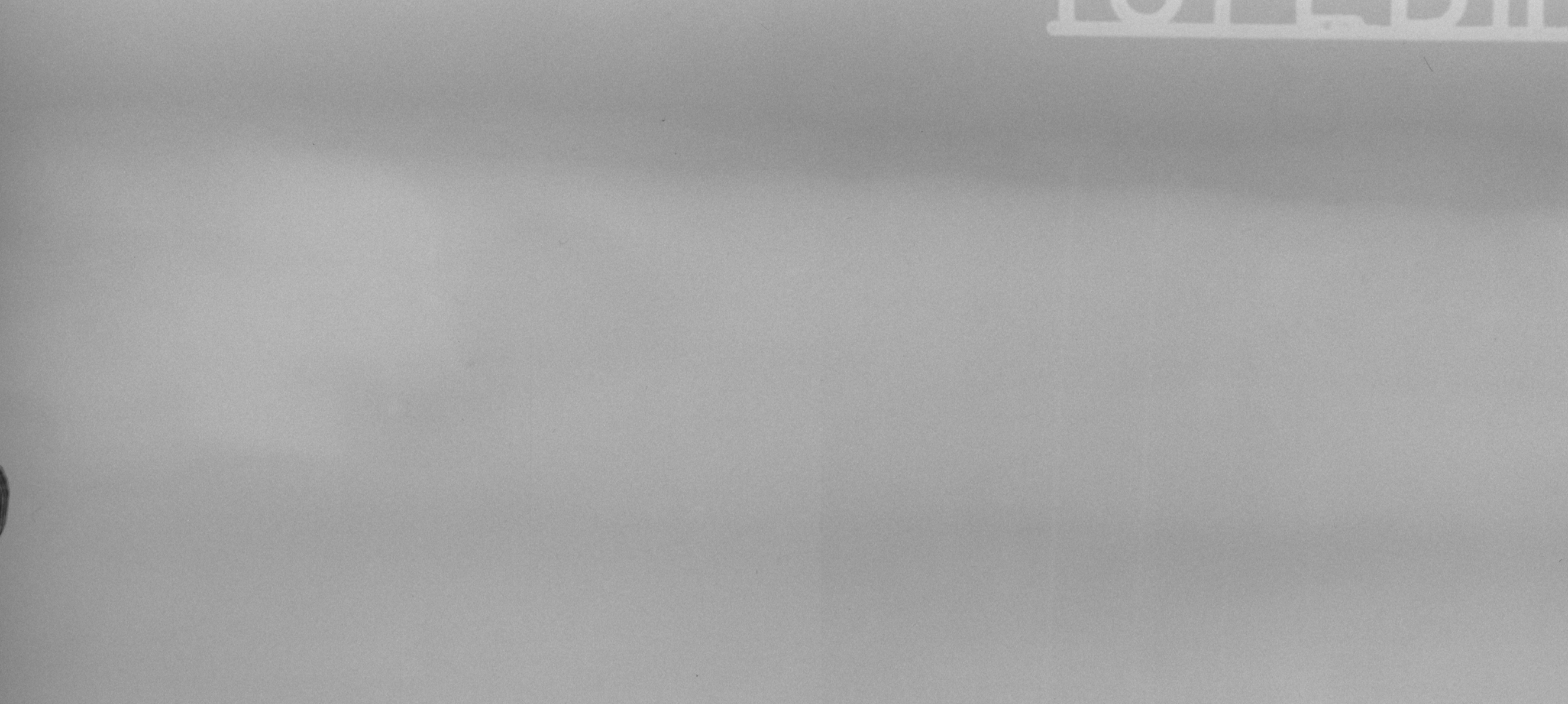
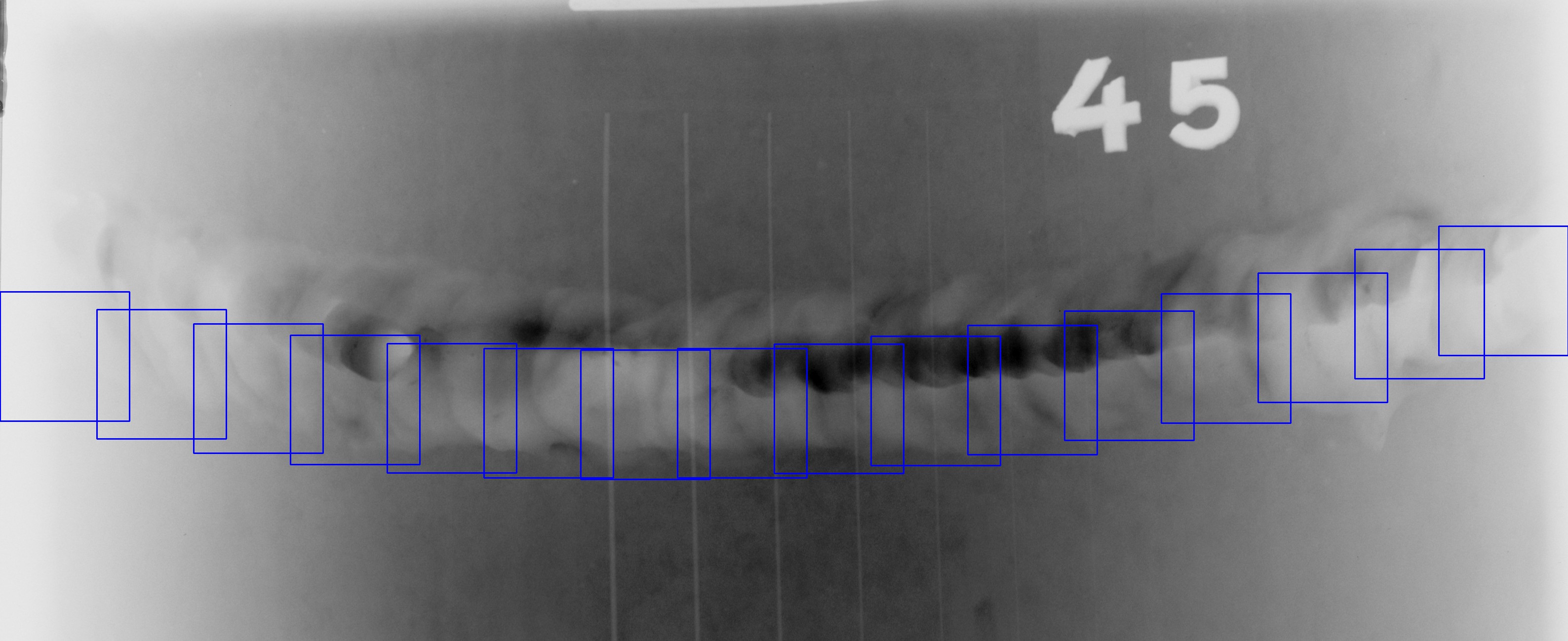
Weak gradient of cleaned seams: If the reinforcement bead is mechanically ground flush or the seam height is minimal (Fig. 2), the difference in optical density between the seam and the pipe metal is only a few brightness units. Simple gradient operators (Sobel, Canny) or global Otsu binarization drown in detector noise.
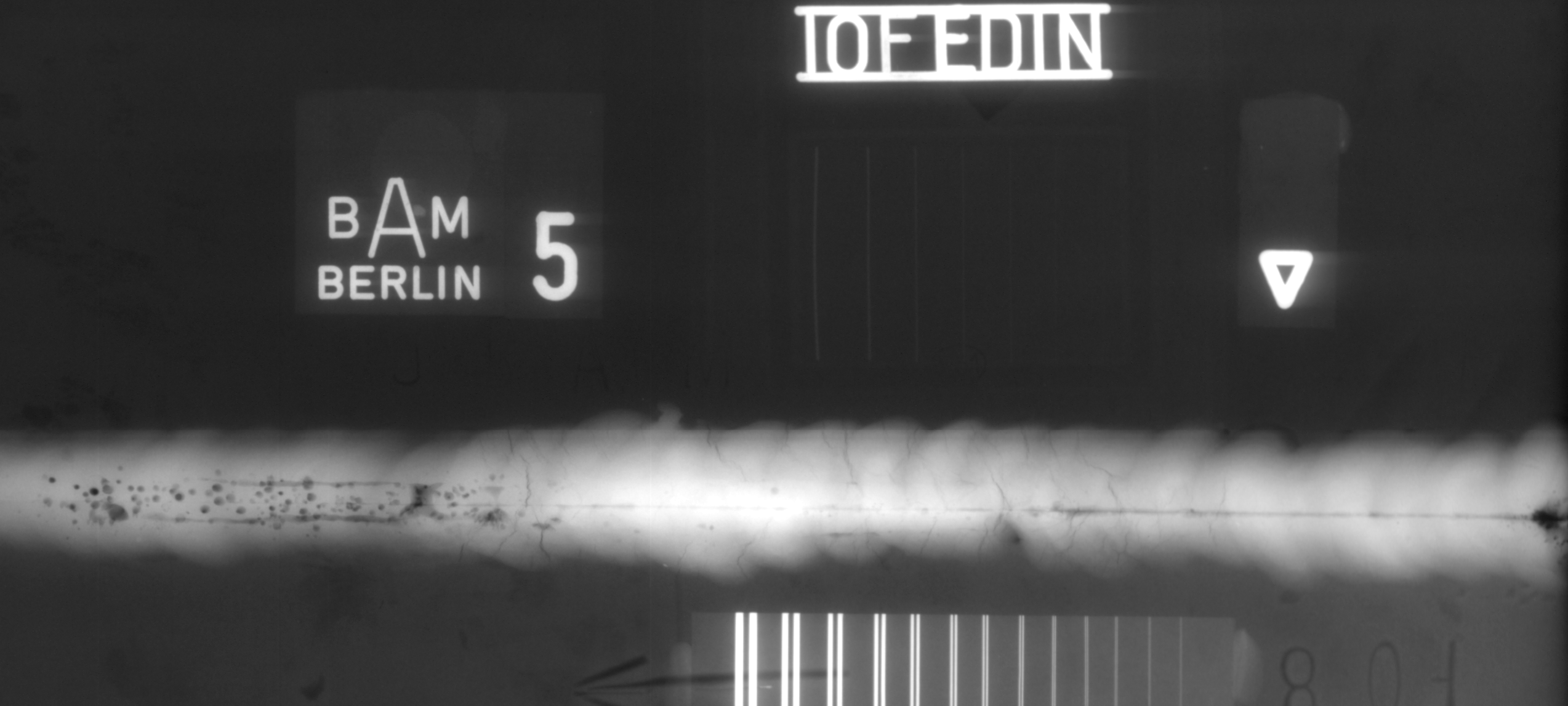
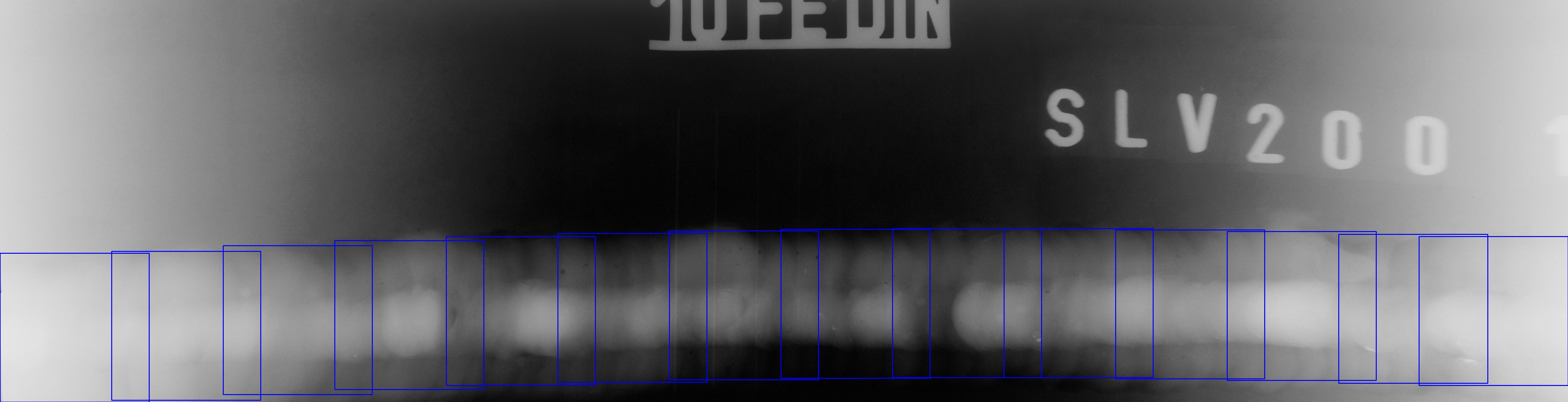
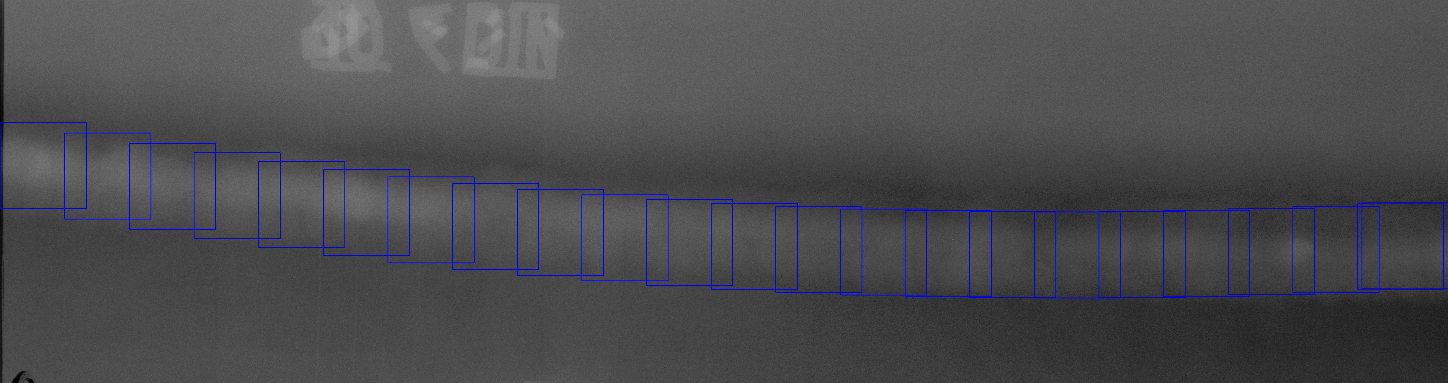
High-contrast markers as a stress test: In real inspection on automated lines, there should be no marking signs on the seam body. However, when designing the algorithm, images with lead letters and wire-type reference standards (Fig. 1) were used deliberately. This served as a harsh stress test: the algorithm must stably extract the seam trajectory and ignore any foreign inclusions of maximum brightness that may occur on the pipe body (technological marks, clamps, metal spatter).

Image of a welded joint from the GDXray W0003 series

Fig. 1. Source image of a welded joint with marking and a reference standard [1]

Low-contrast image with a cleaned weld reinforcement

Fig. 2. Image of a joint with low reinforcement thickness, where the seam is almost indistinguishable by brightness [1]

3. Algorithm for end-to-end tracing and slicing

3.1. Two-pass determination of spatial orientation

The seam in the frame is not required to be strictly horizontal — there are images with vertical joint feed. Attempting to guess the orientation with heuristics is unreliable, so the module performs two independent scanning cycles:

Horizontal pass: The frame is scanned along vertical strips along the X axis. The tracing confidence of the horizontal seam $conf_H$ is calculated.
Vertical pass: The source frame is programmatically rotated 90° clockwise and scanned according to a similar scheme with the calculation of confidence $conf_V$.

If both directions show confidence below 0.5 — the algorithm switches to continuous slicing with a regular grid. If one of the values exceeds the threshold, the dominant direction is selected. In the case when the vertical pass wins ($conf_V > conf_H$), the image is rotated, and further work is carried out in a standardized horizontal plane.

3.2. Suppressing detector noise via 1D integration

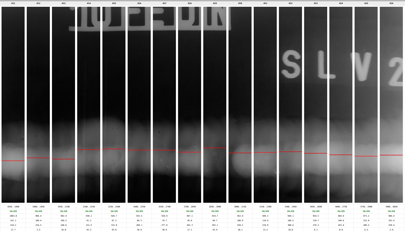
Local noises of the detector matrix are suppressed by an integral method. The image is divided into strips 150 pixels wide. Within each strip, the median profile over rows is calculated:

$$P(y) = \text{median}_{x \in [X_1, X_2]} I(x, y)$$

Fixing the strip width at 150 px guarantees that even a large lead letter or reference wire will occupy no more than 20–25% of the window width. The median filter erases local bursts of marking, restoring the seam profile in the form of a smooth dome.

Diagnostic panorama of strips with the found bead centers

Fig. 3. Diagnostic panorama of vertical strips with fixation of bead extrema

Tracing of the central seam axis with a parabolic spline

Fig. 4. Constructed central seam axis over the source image

3.3. Robust spline approximation: how RANSAC works

After localizing the bead peaks in each strip, an array of coordinate points $(X_i, Y_i)$ is formed. In real images, some of the points inevitably turn out to be false (outliers due to defects in the cassette film, adhered spatter, or edges of the tooling). The ordinary least squares method (OLS) is not applicable here: even one gross outlier with a large leverage radically distorts the shape of the polynomial.

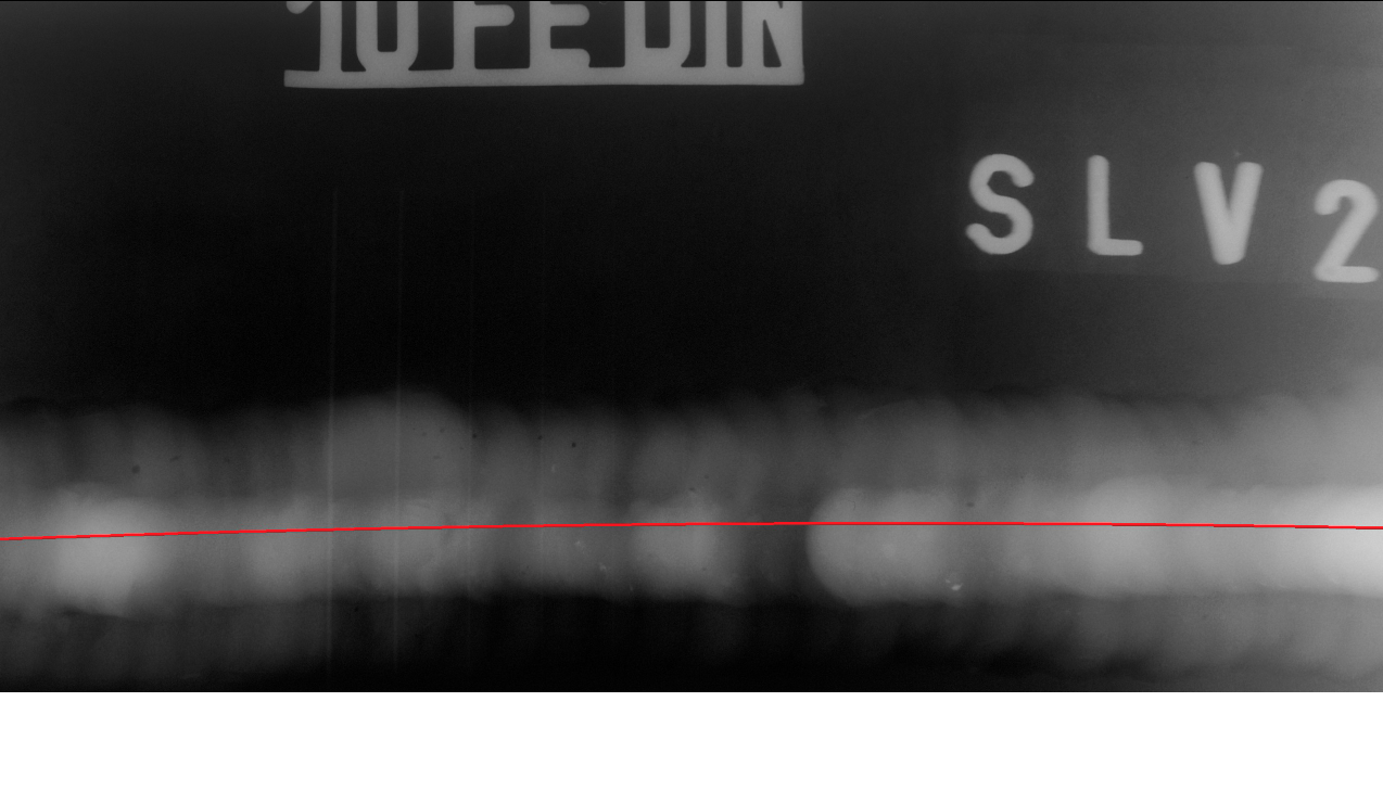
To construct the central seam trajectory, the RANSAC (Random Sample Consensus) algorithm is used [3], adapted for a second-order parabolic spline $Y = ax^2 + bx + c$:

Iterative sampling: From the common pool of points, the minimum necessary set for uniquely constructing a parabola is randomly selected — 3 points. For reproducibility of results, the pseudorandom number generator is initialized with a deterministic seed (seed=42).
Hypothesis formation: An analytical curve is constructed from the selected triplet.
Counting the consensus set (Inliers): For all other points of the array, the absolute residual $|Y_{pred} - Y_i|$ is calculated. Points lying no farther from the curve than a dynamic threshold (5% of the frame height) are assigned to the consensus group (inliers).
Selection of the best model: The procedure is repeated a fixed number of times (150 iterations). The model that collected the largest number of inlier points wins.

The final algorithm confidence ($Confidence$) is calculated as the product of the share of consensus points and the penalty for excessive curvature:

$$Confidence = \frac{N_{inliers}}{N_{total}} \times \max\left(0.0, \, 1.0 - \frac{|a| \cdot W^2}{10 \cdot H}\right)$$

If the points lie on a smooth trajectory of the pipe axis, confidence tends to 1.0. If the points are scattered chaotically, RANSAC rejects the hypothesis, and the confidence value is zeroed.

4. Longitudinal defects and the saddle-shaped profile: a solution via morphology

During testing of the algorithm on images with deep root lack of fusion and through longitudinal cracks, a non-standard edge effect was revealed: the central line on neighboring strips jumped either above or below the defect by 30–50 pixels.

Stepwise jump of centers due to a longitudinal crack

Fig. 5. The problem of splitting the bead profile in the presence of a deep longitudinal discontinuity along the center of the seam

Fig. 6. Correct determination of the extremum after applying one-dimensional grayscale morphological closing

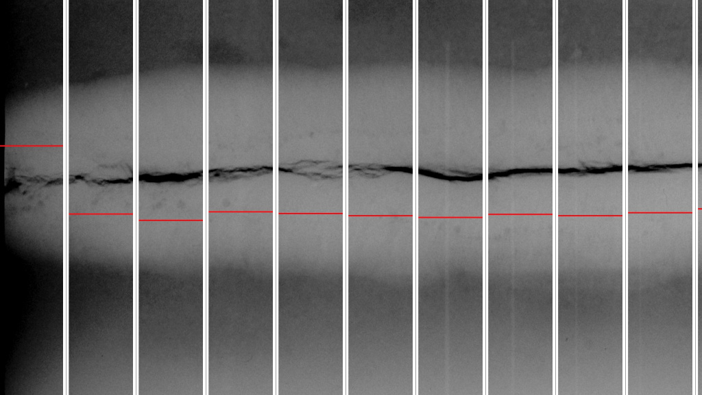
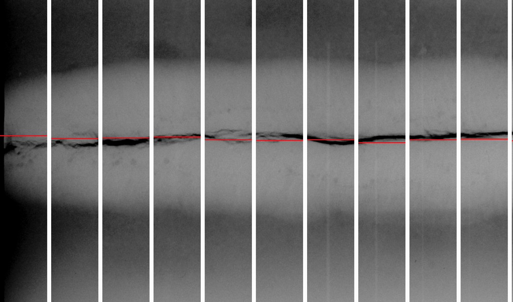
Physical cause: A longitudinal crack creates a band of minimal X-ray attenuation (in the image it looks like a black crevice). As a result, the unimodal light dome of the weld bead splits into two separate hills, forming an M-shaped saddle profile. The classical maximum search clung either to the upper reinforcement bead above the crack or to the lower one.

Mathematical solution: The problem was eliminated by introducing one-dimensional grayscale morphological closing (scipy.ndimage.grey_closing) with a linear structuring element sized ~5% of the frame height. Vertical closing effectively "fills" the dark dip of the crack with the values of the surrounding optical density of the weld metal. The split profile restores monotonicity, and the true center of the joint is calculated as the geometric midpoint at the half-height of the bead (FWHM).

5. Software implementation

Below is the key block of profile analysis and assembly of the RANSAC approximation:

from typing import Any, Dict, List, Optional, Tuple
import cv2
import numpy as np
from scipy.ndimage import gaussian_filter1d, grey_closing
from scipy.signal import find_peaks

def analyze_direction(
    gray_img: np.ndarray, stripe_width: int = 150
) -> Tuple[float, Optional[np.ndarray], float, List[Dict[str, Any]]]:
    """Profile analysis with morphological crack closing and RANSAC spline."""
    h, w = gray_img.shape
    eff_w = min(stripe_width, w)

    stripe_ranges = []
    x = 0
    while x + eff_w <= w:
        stripe_ranges.append((x, x + eff_w))
        x += eff_w
    if not stripe_ranges or stripe_ranges[-1][0] < (w - eff_w):
        stripe_ranges.append((w - eff_w, w))

    global_row_med = np.median(gray_img, axis=1)
    global_smooth = gaussian_filter1d(global_row_med, sigma=max(3, h // 30))
    y_global_hint = int(np.argmax(global_smooth))
    dyn_range = float(np.max(global_smooth) - np.min(global_smooth))

    x_coords, y_coords, seam_widths = [], [], []
    sigma_val = max(3.0, h / 35.0)
    closing_size = max(15, int(h * 0.05))

    for x1, x2 in stripe_ranges:
        stripe_raw = gray_img[:, x1:x2]
        prof = np.median(stripe_raw, axis=1)

        # Morphological closing: "stitching" M-shaped dips from cracks
        closed_prof = grey_closing(prof, size=closing_size)
        smooth = gaussian_filter1d(closed_prof, sigma=sigma_val)

        min_w = max(5, int(h * 0.05))
        prominence = max(4.0, dyn_range * 0.15)
        peaks, props = find_peaks(smooth, prominence=prominence, width=min_w)

        if len(peaks) > 0:
            best_idx = int(np.argmin(np.abs(peaks - y_global_hint)))
            # Geometric center by FWHM excludes a shift toward one of the beads
            left_ip = props["left_ips"][best_idx]
            right_ip = props["right_ips"][best_idx]
            chosen_y = float((left_ip + right_ip) / 2.0)

            x_coords.append((x1 + x2) / 2.0)
            y_coords.append(chosen_y)
            seam_widths.append(float(props["widths"][best_idx]))

    num_stripes = len(stripe_ranges)
    if len(x_coords) < num_stripes * 0.3:
        return 0.0, None, 0.0, []

    # Deterministic RANSAC (seed=42)
    rng = np.random.default_rng(42)
    xs, ys = np.array(x_coords), np.array(y_coords)
    best_inliers, best_poly = 0, None
    threshold = max(8.0, h * 0.05)

    for _ in range(150):
        if len(xs) < 3:
            break
        idx = rng.choice(len(xs), 3, replace=False)
        try:
            poly = np.polyfit(xs[idx], ys[idx], 2)
        except np.linalg.LinAlgError:
            continue
        inliers = np.sum(np.abs(np.polyval(poly, xs) - ys) < threshold)
        if inliers > best_inliers:
            best_inliers = inliers
            best_poly = poly

    if best_poly is None:
        return 0.0, None, 0.0, []

    curv_penalty = max(0.0, 1.0 - abs(best_poly[0]) * (w**2) / (h * 10.0))
    confidence = float(np.clip((best_inliers / float(num_stripes)) * curv_penalty, 0.0, 1.0))
    median_width = float(np.median(seam_widths)) if seam_widths else float(h * 0.15)

    return confidence, best_poly, median_width, []

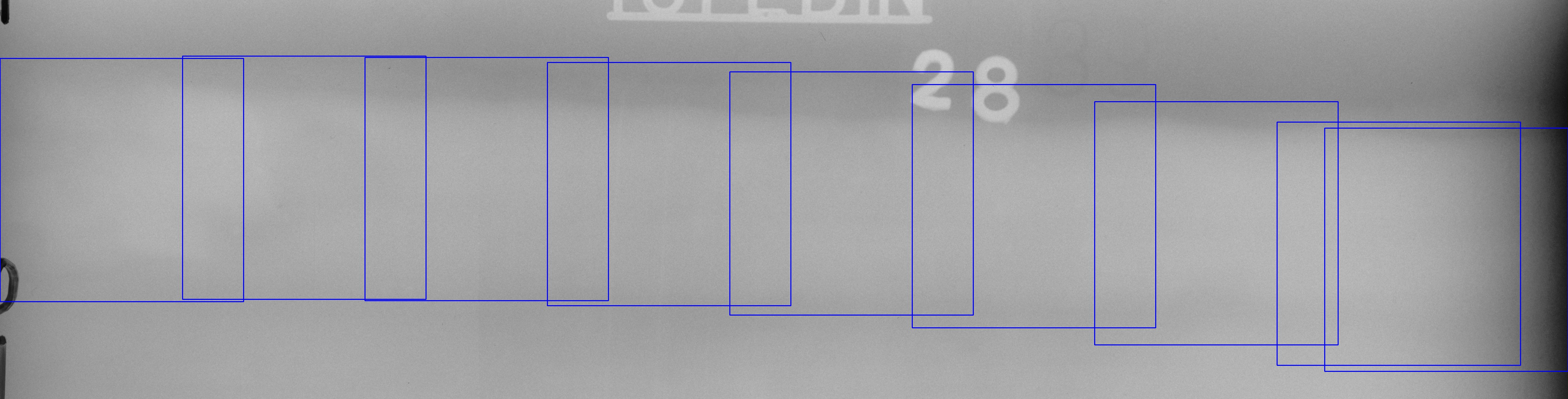
6. Examples of resulting patch layouts with guaranteed capture of the seam and the near-seam zone

Final layout of slices along the seam contour

Fig. 7. Correct result on a complex scenario (rather low contrast of the seam relative to the pipe body)

Fig. 8. Any reference standards and high-brightness inscriptions are ignored

Fig. 9. An arched seam is not a problem

Fig. 10. Here the result is not entirely good, although close. There is room for improvement.

Conclusions

The quality of a convolutional neural network in radiographic testing is laid down at the stage of dataset formation. Attempts to mechanically slice frames with a dense sliding window followed by random splitting lead to fictitious overfitting, hidden data leakage, and the inability of the model to find real defects on new joints.

The proposed approach based on bidirectional projection profiling, one-dimensional morphological closing, and deterministic spline RANSAC ensures stable seam tracing even with pronounced longitudinal defects, a cleaned bead, and the presence of marking signs. The formed slices are centered relative to the real joint axis and include both the seam body and the near-seam space, which allows training detection models on physically correct data.

References and sources

GDXray: The Database of X-ray Images for Nondestructive Testing
Domingo Mery, Vladimir Riffo, Uwe Zscherpel, German Mondragón, Iván Lillo, Irene Zuccar, Hans Lobel, Miguel Carrasco
Journal of Nondestructive Evaluation, Vol. 34, No. 4, Art. 42, 2015. DOI: 10.1007/s10921-015-0315-7.
Project repository: https://github.com/computervision-xray-testing/GDXray
📄 Download the article: 2015_GDXray.pdf

Anatomy of the RIAWELC dataset. A useful project or pseudo-academic concoction?
Publication: https://dps.com.ru/posts/ru/what_RIAWELC_really_is.html

Random Sample Consensus: A Paradigm for Model Fitting with Applications to Image Analysis and Automated Cartography
Fischler M. A., Bolles R. C.
Communications of the ACM, Vol. 24, No. 6, 1981, pp. 381–395. DOI: 10.1145/358669.358692.

Additional materials

Example report of my slicer implementation:
📄 W0003_0020_report.html (Caution, the file is large ~7.7 MB)